(Difference between revisions)
| Revision as of 12:10, 15 September 2006 Peter (Talk | contribs) (→Calibrating Yield) ← Previous diff |
Revision as of 12:11, 15 September 2006 Peter (Talk | contribs) (→Finding the relevant parameters with a principle component analysis) Next diff → |
||
| Line 21: | Line 21: | ||
| ===Finding the relevant parameters with a principle component analysis=== | ===Finding the relevant parameters with a principle component analysis=== | ||
| - | + | {|"class=prettytable" cellpadding="15" border="1" style="border-collapse:collapse" | |
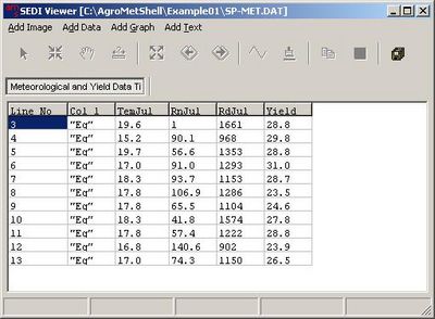
| + | |width="300"|To illustrate how principal component analysis can be used, examine the input file SP-MET.DAT. The file contains annual yield from 1920 to 1930 and three climatological variables; the mean temperature, precipitation and radiation measured during the month of July. We imagine that the yield is a function of these three parameters but we suspect that the three variables are not entirely independent of one another. | ||
| + | ||[[Image:graph84.jpg|400px|]] | ||
| + | |---- | ||
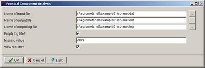
| + | |width="300"|Activate the ''Tools - Principle Component Analysis'' function. A settings window appears.||[[Image:graph85.jpg|400px|]] | ||
| + | |---- | ||
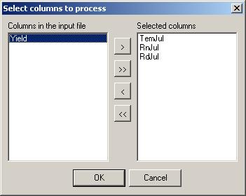
| + | |width="300"|Select the variables you want to work with. For this example, select the variables TemJul, RnJul and RdJul. Clicking on the Ok button will start the calculations.||[[Image:grap86.jpg|grap86.jpg]] | ||
| + | |---- | ||
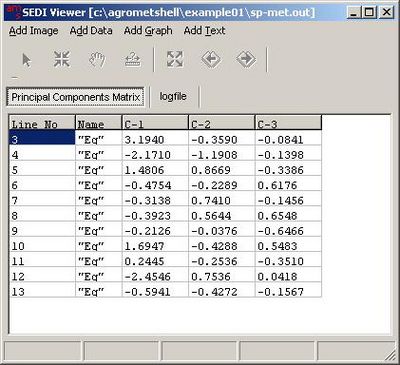
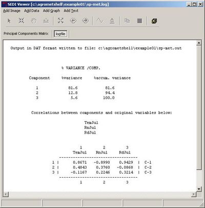
| + | |width="300"|The output from the analysis is presented in two ways: as an output file, containing the values of the principal components themselves.||[[Image:graph87.jpg|400px|]] | ||
| + | |---- | ||
| + | |width="300"|This information allows you to interpret the results and determine which variables can be used in the regression model. The log file lists the variables, their extreme values and the % of variance explained by each component. This is followed by the accumulated variance of each component and a correlation matrix. This information tells us that the first and second principal components together explain 94.4% of the total variance and the third component can therefore be discarded. Geometrically, this means that all the observed points find themselves on a plane and 94.4% of the variation is parallel to this plane while 5.6% is perpendicular to it. In addition, 81.6% of the variation corresponds to the principal component and only 18.5% to the other two. The second and third components can therefore be discarded.||[[Image:graph88.jpg|400px|]] | ||
| + | |} | ||
Revision as of 12:11, 15 September 2006
Calibrating Yield
The yield function is a statistically derived function relating the water balance parameters (which constitute the outputs of the water balance model) and the other factors (farm inputs, trend) or NDVI with station yield. Once this function has been established, it can be used for early crop yield forecasting.
Although many different equations are possible, the most widely used one is the outcome of a multiple linear regression procedure:
Y = a + b1X1 + b2X2 + b3X3where b1 to b3 are the corresponding X coefficients.
Using an example for Malawi, first it will be established which water balance parameters are good predictors for yield. Then the multiple linear regression will be performed.
The input data file for Malawi contains multiple lines for stations and years. In every line, besides yield, all possibly relevant water balance output parameters are stored. The file can be downloaded here 
Finding the relevant parameters with a principle component analysis

